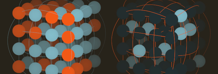
High-dimensional graph-based models with discrete random variables (e.g. Boltzmann machines, Markov networks, Ising models, Potts models) all require an algorithm in order to generate random samples. Each algorithm possesses different properties and tradeoffs, making it difficult to know which method is the best choice. I decided to develop a program to help me gain intuition in this domain.

Sample Lab is a workbench for comparing sampling algorithms for discrete graph-based models under various conditions. This page gives a brief overview of the program options and a few sampling algorithms.
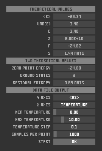
The UI is partitioned into model options, simulation options, empirical values, theoretical values, zero temperature theoretical values, and data file output:
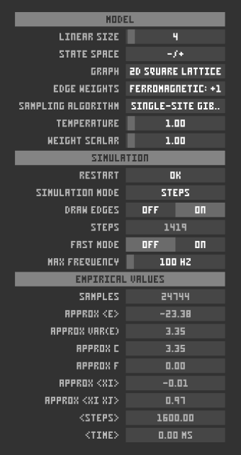
Model options include:
For example, these images of triangular graphs show a few combinations of Ising vs. Boltzmann state spaces and ferromagnetic vs. antiferromagnetic edge weights:
Here are square graphs with Boltzmann states comparing ferromagnetic and antiferromagnetic edge weights:
And here are cube graphs with Ising states comparing ferromagnetic and antiferromagnetic edge weights:
The simulation/visualization options are fairly self-explanatory. Empirical values are computed in real time by averaging over the current set of completed samples. Theoretical values are computed whenever the model options change. (But most of these values depend on the normalizing constant Z, which is incomputable for all but the smallest models, so we only compute these for models with <= 16 nodes.) The zero temperature theoretical values are useful when studying that special case.
Data files can be generated to be fed to an external plotting program. X axis options are temperature or model size, and Y axis can be energy mean, energy variance, heat capacity, average computational steps per sample, and average elapsed milliseconds per sample. The X axis is incremented automatically through the chosen range, and a number of samples are generated at each step and used to compute and output averages.
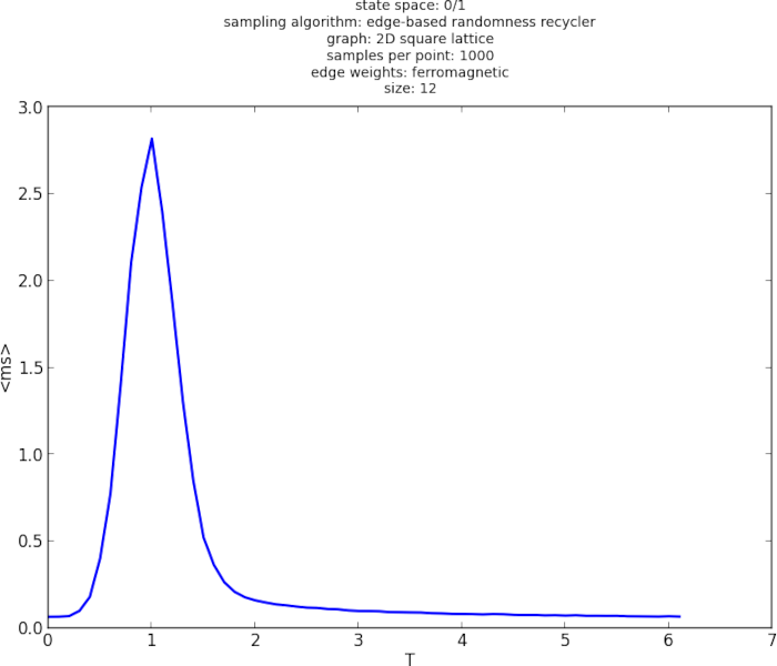
For example, here is a plot of measured runtime (ms/sample) over temperature, showing a definite peak at a critical temperature value:
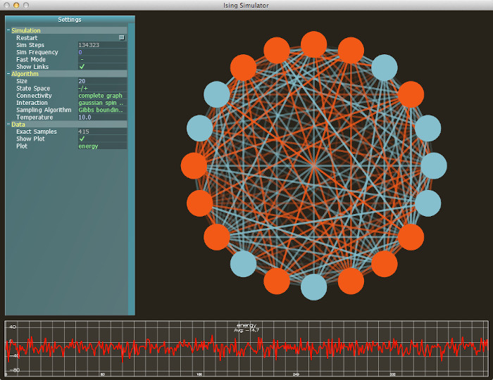
In an older version, I had real-time plots generated directly, but I ended up needing to plot data externally anyway, so I removed the feature. Here is a screenshot of the old version:
The simplest algorithm, Gibbs sampling, is a MCMC method which is easy to implement but lacks certain guarantees. In particular, it is difficult to know when the Gibbs sampler's Markov chain has converged, at which point the sample is a valid draw from the model's equilibrium distribution. The video here shows a triangular graph with Boltzmann states and antiferromagnetic edge weights. There is no specific point where it is clear that the Markov chain has converged.
So-called "perfect sampling" or "exact sampling" algorithms are methods that guarantee equilibrium samples. One well-known approach is coupling from the past (CFTP), which is described well in MacKay's book (ch.32). CFTP conceptually starts a separate Markov chain in every possible state of the system and waits for them all to merge/coalesce into a single chain. These chains are started at some predetermined time step in the past, and if coalescence hasn't happened by t=0, we start the process again further into the past, but using the same random number sequence at each time step as before. This overall process continues until coalescence occurs, at which point the sample is valid.
Note that it would be impractical to store and track all possible Markov chains explicitly (consider the number of initial states of a system with N binary variables). Instead, CFTP methods simply track a set of bounds on the states of the system and detect when the bounds collapse to a single state. These bounds can be simple for highly restricted cases. The "bounding chain" method of Mark Huber is a general bounding method which works for binary node states and any real-valued edge weights. This method adds a separate "unknown" state to each node (indicated in white in the video here). When all of these unknowns disappear, all of the Markov chains have coalesced into a single chain.
Another method is the "edge-based randomness recycler," also by Mark Huber. This constructs a sample by starting with a fully disconnected graph and attempting to incorporate one edge at a time. Specifically, at each step it considers a node that is not yet part of the current collection, generates a random state for it, and uses the edge weights from that node to determine whether to accept the new addition. If, at any step, the new addition is rejected, only a part of the current collection is reset, essentially "recycling" much of the previous work without starting over from scratch.